| 일 | 월 | 화 | 수 | 목 | 금 | 토 |
|---|---|---|---|---|---|---|
| 1 | 2 | 3 | ||||
| 4 | 5 | 6 | 7 | 8 | 9 | 10 |
| 11 | 12 | 13 | 14 | 15 | 16 | 17 |
| 18 | 19 | 20 | 21 | 22 | 23 | 24 |
| 25 | 26 | 27 | 28 | 29 | 30 | 31 |
- mnist
- 합성곱 신경망
- 소수
- 역전파
- 냥코 센세
- Gram matrix
- 역전파법
- CNN
- 전처리
- 소인수분해
- Convolutional Neural Network
- neural network
- 신경망
- Autoencoder
- 자전거 여행
- deep learning
- 오일러 프로젝트
- backpropagation
- 비샤몬당
- 수달
- A Neural Algorithm of Artistic Style
- 베이지안
- 오토인코더
- bayesian
- c#
- 딥러닝
- project euler
- 히토요시
- SQL
- Python
- Today
- Total
통계, IT, AI
딥러닝: 화풍을 모방하기 (4) - 연습: 회귀 문제 본문
1. 개요
- 다음 파트로 넘어가기 전에 지금까지 배운 것을 구현하여 이해를 확실하게 하자.
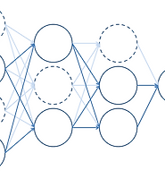
- 가장 간단한 경우부터 연습하기 위하여 변수가 1개인 회귀 문제를 선택한다. 즉, 신경망은 다음과 같다.

- 출력층의 활성함수는 항등함수로 한다. 그러므로 \(u_1=w_{11}x_1+b_1\)이며 \(z_1=f(u_1)=u_1\)이다.
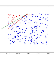
- 연습에 사용할 \(x_1\)은 \(U(-4,4)\)에서 200개를 생성한다.
- 출력 \(d\)는 \(x_1-1+\varepsilon\)이며 \(\varepsilon\)은 \(N(0,1)\)를 따른다.
- 데이터의 형태는 그림 2와 같다. 붉은 선은 연습에서 추정해야 할 파라미터를 나타낸다.

- minibatch를 사용하며 1개의 batch size는 20으로 하며 반복횟수(epoch)는 2,000으로 한다.
- 테스트 데이터는 연습데이터에서 임의로 20개를 골라 사용한다.
- 오차 함수는 제곱오차를 사용한다.
$$E(\boldsymbol{w})=\frac{1}{2}\sum_{i=1}^{N}\left\| y(x_i;\boldsymbol{w})-d_i\right\|^2$$
- 따라서 파라미터의 미분은 다음과 같다.
$$\frac{\partial E}{\partial \boldsymbol{w}}=\frac{\partial E}{\partial w_{11}}=\sum_{i \in D_t}(y(x_i;\boldsymbol{w})-d_i)x_{1i}, \quad \frac{\partial E}{\partial \boldsymbol{b}}=\frac{\partial E}{\partial b_{1}}=\sum_{i \in D_t}(y(x_i;\boldsymbol{w})-d_i) $$
2. 구현
- 파이썬을 사용하여 구현하며, numpy, matplotlib와 같은 패키지를 사전에 깔아둔다.
- 가능한 매트릭스 연산을 사용하여 코드를 간결하게 하며 계산 속도를 높인다.
# -*- coding: utf-8 -*-
import numpy as np
import matplotlib.pyplot as plt

""" GENERAL SETTING """
np.random.seed(0)
enable_visualization = True


""" DATA """
N = 200
x_1 = np.random.uniform(-4, 4, N)
W = np.array([-1, 1]).reshape((-1,1)) # uppercase of w is target parameter
d = np.column_stack(([1]*N,x_1)).dot(W) + np.random.normal(0, 1, N).reshape((N,1))
X = np.column_stack((x_1)).reshape((N,1))

test_data_index = np.random.randint(N, size=20)
test_x = X[test_data_index,]
test_d = d[test_data_index,]

if enable_visualization:
    plt.plot(x_1, d, 'bo')
    plt.plot(np.array([-4,4]), np.array([[1,-4],[1,4]]).dot(W), color='red')
    plt.show()


""" FUNCTION """
def activate(u, type='i'):
    if type == 'i':
        return u

def feedforward(X, w, b):
    X = np.column_stack(([1]*X.shape[0], X))
    w = np.vstack((b,w))
    return activate(X.dot(w))

def error(X, w, b, d, feedforward):
    return np.linalg.norm(feedforward(X, w, b) - d)**2/2

""" PARAMETER & OPTIMIZATION SETTINGS """
w = np.array([0.0]).reshape((-1,1))
b = np.array([0.0]).reshape((-1,1))
epsilon = 0.001
batch_size = 20  # number of samples in minibatch
epoch_size = 2000

error_history = [error(test_x, w, b ,test_d, feedforward)]
index_list = np.arange(0,N)


""" OPTIMIZATION """
for epoch in range(epoch_size):
    np.random.shuffle(index_list)

    for i in range(N//batch_size):
        training_index = index_list[(i*batch_size):((i+1)*batch_size)]

        training_x = X[training_index,]
        training_d = d[training_index,]

        # Caculate nabla E
        der_error = feedforward(training_x, w, b) - training_d
        der_w, der_b = np.mean(der_error*training_x, axis=0), np.mean(der_error, axis=0)
        der_w, der_b = np.asmatrix(der_w).reshape((-1,1)), np.asmatrix(der_b).reshape((-1,1))

        w -= epsilon * der_w
        b -= epsilon * der_b

    error_history.append(error(test_x, w, b ,test_d, feedforward))


""" RESULT """
if enable_visualization:
    # OPTIMIZATION
    plt.plot(x_1, d, 'bo')
    plt.plot(np.array([-4,4]),
             np.array([[1,-4],[1,4]]).dot(W), color='red')
    plt.plot(np.array([-4,4]),
             np.array([[1,-4],[1,4]]).dot(np.vstack((b,w))), color='green')
    plt.show()

    # ERROR HISTORY
    plt.plot(error_history)
    plt.show()

print( b, w)
3. 결과
- \(b\)와 \(w_{11}\)의 추정치는 각각 -1.11, 0.95이며 아래 그림의 초록 선으로 나타낼 수 있다.

- 아래는 반복 횟수에 따른 테스트오차의 경향이다. 500회를 반복하기 전에 학습을 끝내도 됬다는 것을 알 수 있다.

'머신러닝' 카테고리의 다른 글
| 딥러닝: 화풍을 모방하기 (6) - 연습: 다클래스 분류 문제 (1) | 2017.02.02 |
|---|---|
| 딥러닝: 화풍을 모방하기 (5) - 연습: 이진 분류 문제 (0) | 2017.02.01 |
| 딥러닝: 화풍을 모방하기 (3) - 책 요약: 3. 확률적 경사 하강법 (1) | 2017.01.30 |
| 딥러닝: 화풍을 모방하기 (2) - 책 요약: 2. 앞먹임 신경망 (0) | 2017.01.30 |
| 딥러닝: 화풍을 모방하기 (1) - 책 요약: 1. 시작하며 (0) | 2017.01.27 |